Predict Fastest Speed

Apply Machine Learning Algorithm to Predict Fastest Lap Speed in Formula One Race

Formula One (F1) is the most prestigious single-seater car race in the world. One season in F1 consists of multiple races that take place around the world at special F1 circuits and on public roads.

I applied classic linear regression model to predict fastest lap speed - fastest lap speed is important to consider in a F1 race, since the faster one is, the shorter it takes. With lots of advertisement and sponsoring going on this event, it is a good arena for manufacturers to showcase their machinery.

As with all machine learning models, it first starts with preparing the data. For this analysis, I merged four different tables to create a master dataset to create the final dataset.

Step 1: Prepare Data

The codes are written in python script in databricks environment. Data is called from Amazon Web Services (AWS).

To predict fastest lap speed, using driver information (driver age), circuit information (circuit location; i.e. latitude and longitude), and race information (points earned, rank, position, grid, raceId, number of laps, the driver’s rank at that race)

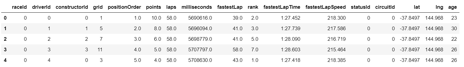
I merged four different datasets using different aliases. Below is a snippet of output data frame.

Step 2: Check Assumptions

Two biggest assumptions that need to be satisfied when creating a linear regression model are (relative) normal distribution of the dependent variable and linear relationship between the independent variables and the dependent variable.

I first plotted histogram of fastest lap speed (dependent variable) to see if the distribution displays a relatively normal distribution.

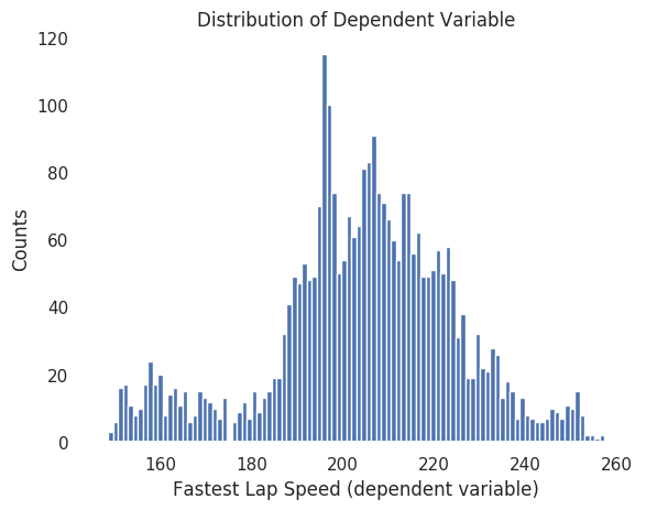
Thankfully, the histogram shows approximate normal distribution.

I also created a correlation plot, colored with a heatmap to see correlation. Choosing independent variables equate to selecting features in a machine learning model. Machine learning algorithm will use these features (or independent variables) to optimize on predicting the outcome (or dependent variable).

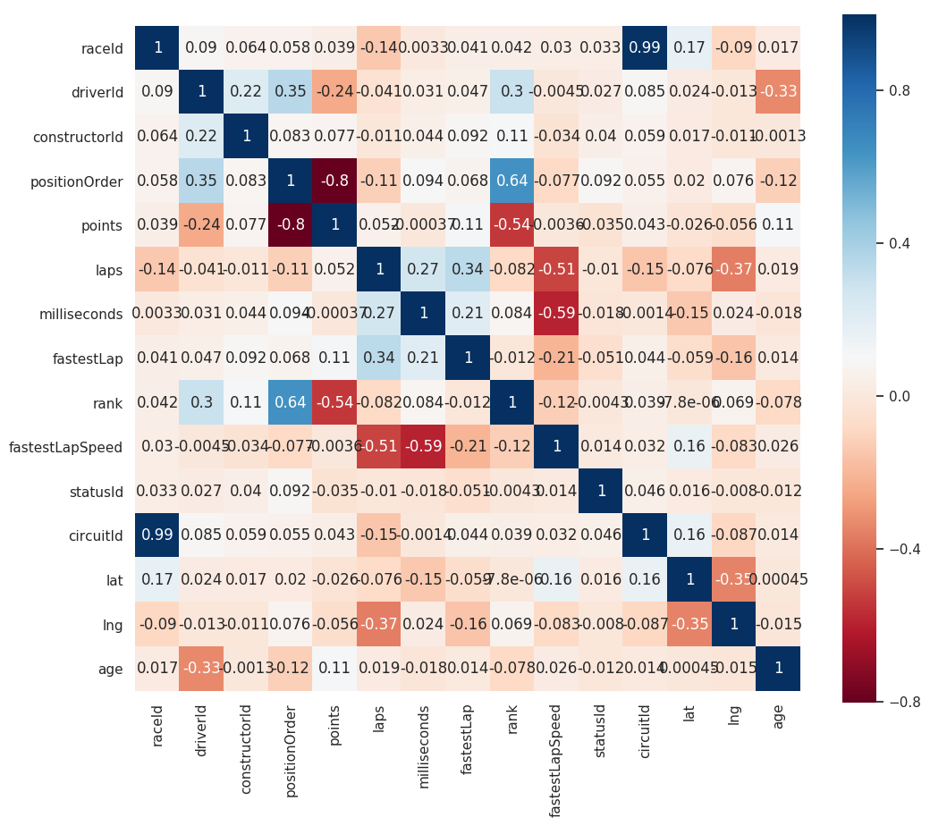
Linear relationship is not absent in this model - maybe a good linear regression model will work.

Step 3: Select Features

When the number of features is too many, visualization may not be the easiest way to find out correlation. Hence, one can filter and select values with absolute correlation over a certain number.

Example python script will be like below.

corr_values = abs(df.corr()['dep_var_col'])
corr_values[corr_values > 0.2] # alter the number

I chose milliseconds, laps, fastestLap, rank, lat to predict fastestLapSpeed.

Step 4: Split Data, Run Experiment Model

As with all machine learning processes, I split the data to training and testing sets with ratio of 7:3. sklearn package was used.

Then, I ran the model. Even though I used a linear regression, I thought adding penalization terms will improve the model. sklearn has ridge and lasso penalizations available for linear regression. The alpha levels range from 0 to 1.

Results of the naive model using ridge penalization set to alpha level of 0.4 yielded this result.

# Root Mean Squared Error: 15.191144501367365
# R_squared: 0.42471455742528186

This is the residual plot.

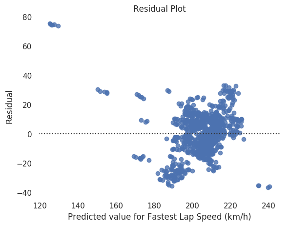
Residual plot is scattered and is not orderly. Also, root mean squared error and R-squared value is quite good; maybe changing penalizations could improve the model.

Step 5: Select the Best Model

To improve my predictive model, I tried varying alpha levels from 0.1 to 1 on lasso and ridge penalizations. When alpha level on lasso increases, model behaves less like ordinary least squares and ignore less important features. So, when doing lasso penalization, I also made sure to record how many features are used.

Moreover, I also specified the model to normalize to improve model performance.

When I ran multiple models, the best model was ridge model with alpha of 0.3 and normalization as True. Normalized values are better because for this regression, all variables have different distribution. Normalization improves model performance by regularizing weight placed on each of the variables. But, as with penalization, larger alpha makes the model less flexible; hence, a larger alpha (0.4 or more) is not as effective as alpha level at 0.3. By fine tuning the alpha levels from 0.26 to 0.32, all perform less than at alpha level of 0.3, which shows that alpha at 0.3 suits best in this case.

• Note: Link to the codes and process is available here